Section: 17 🔖 Predictions with rpart
17.1 Introduction
Decision trees are one of the most powerful and popular tools for classification and prediction. The reason decision trees are very popular is that they can generate rules which are easier to understand as compared to other models. They require much less computations for performing modeling and prediction. Both continuous/numerical and categorical variables are handled easily while creating the decision trees.
17.2 Use of Rpart
Recursive Partitioning and Regression Tree RPART library is a collection of routines which implements a Decision Tree.The resulting model can be represented as a binary tree. For the purpose of illustration of rpart we will continue to use data puzzle 3.1 set - the Professor Moody data set.
The library associated with this RPART is called rpart. Install this library using install.packages("rpart").
Syntax for building the decision tree using rpart():
rpart( formula , method, data, control,...)- formula: here we mention the prediction column and the other related columns(predictors) on which the prediction will be based on.
prediction ~ predictor1 + predictor2 + predictor3 + ...
- method: here we describe the type of decision tree we want. If nothing is provided, the function makes an intelligent guess. We can use “anova” for regression, “class” for classification, etc.
- data: here we provide the dataset on which we want to fit the decision tree on.
- control: here we provide the control parameters for the decision tree. Explained more in detail in the section further in this chapter.
- formula: here we mention the prediction column and the other related columns(predictors) on which the prediction will be based on.
For more info on the rpart function visit rpart documentation
Lets look at an example on the Moody 2022 dataset.
- We will use the rpart() function with the following inputs:
- prediction -> GRADE
- predictors -> SCORE, DOZES_OFF, TEXTING_IN_CLASS, PARTICIPATION
- data -> moody dataset
- method -> “class” for classification.
17.2.1 rpart()
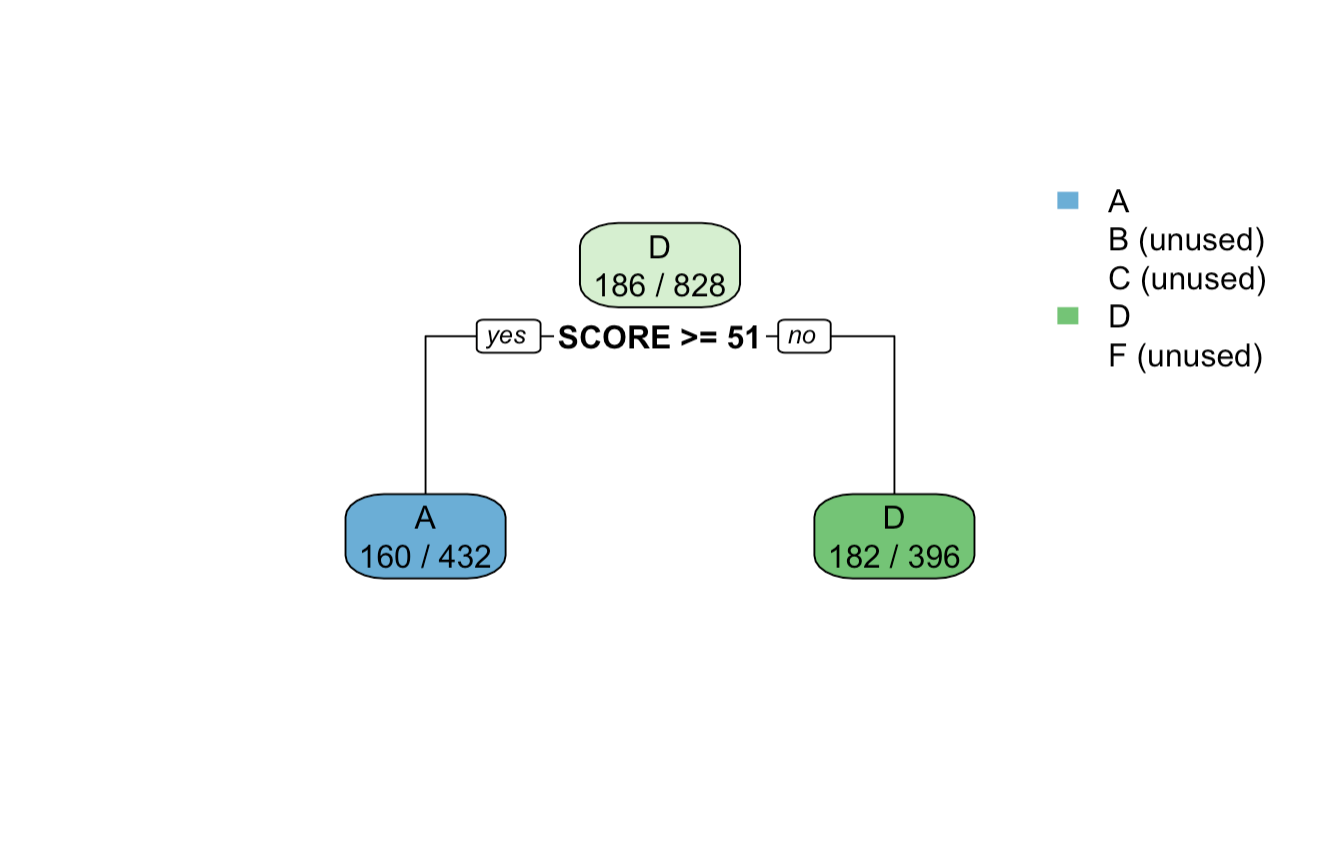
We can see that the output of the rpart() function is the decision tree with details of,
- node -> node number
- split -> split conditions/tests
- n -> number of records in either branch i.e. subset
- yval -> output value i.e. the target predicted value.
- yprob -> probability of obtaining a particular category as the predicted output.
Using the output tree, we can use the predict function to predict the grades of the test data. We will look at this process later in section 17.6
But coming back to the output of the rpart() function, the text type output is useful but difficult to read and understand, right! We will look at visualizing the decision tree in the next section.
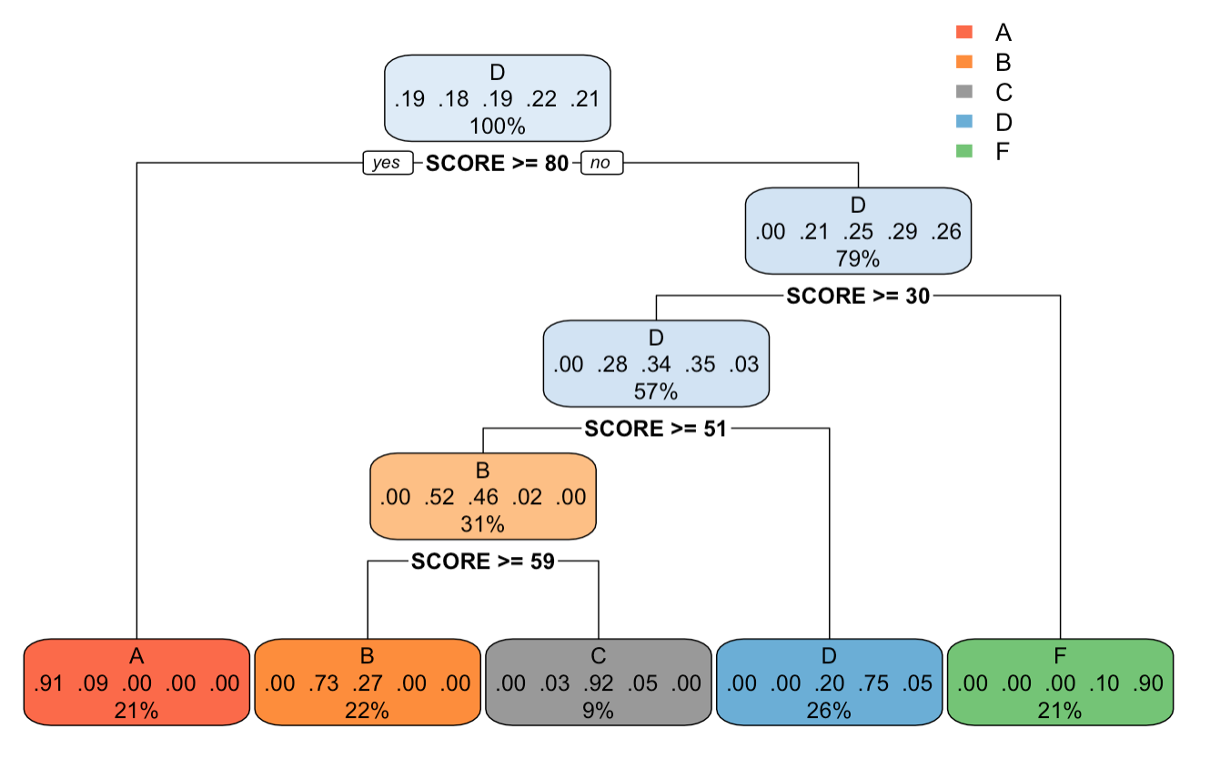
17.3 Visualize the Decision tree
To visualize and understand the rpart() tree output in the easiest way possible, we use a library called rpart.plot. The function rpart.plot() of the rpart.plot library is the function used to visualize decision trees.
NOTE: The online runnable code block does not support rpart.plot library and functions, thus the output of the following code examples are provided directly.
17.3.1 rpart.plot()
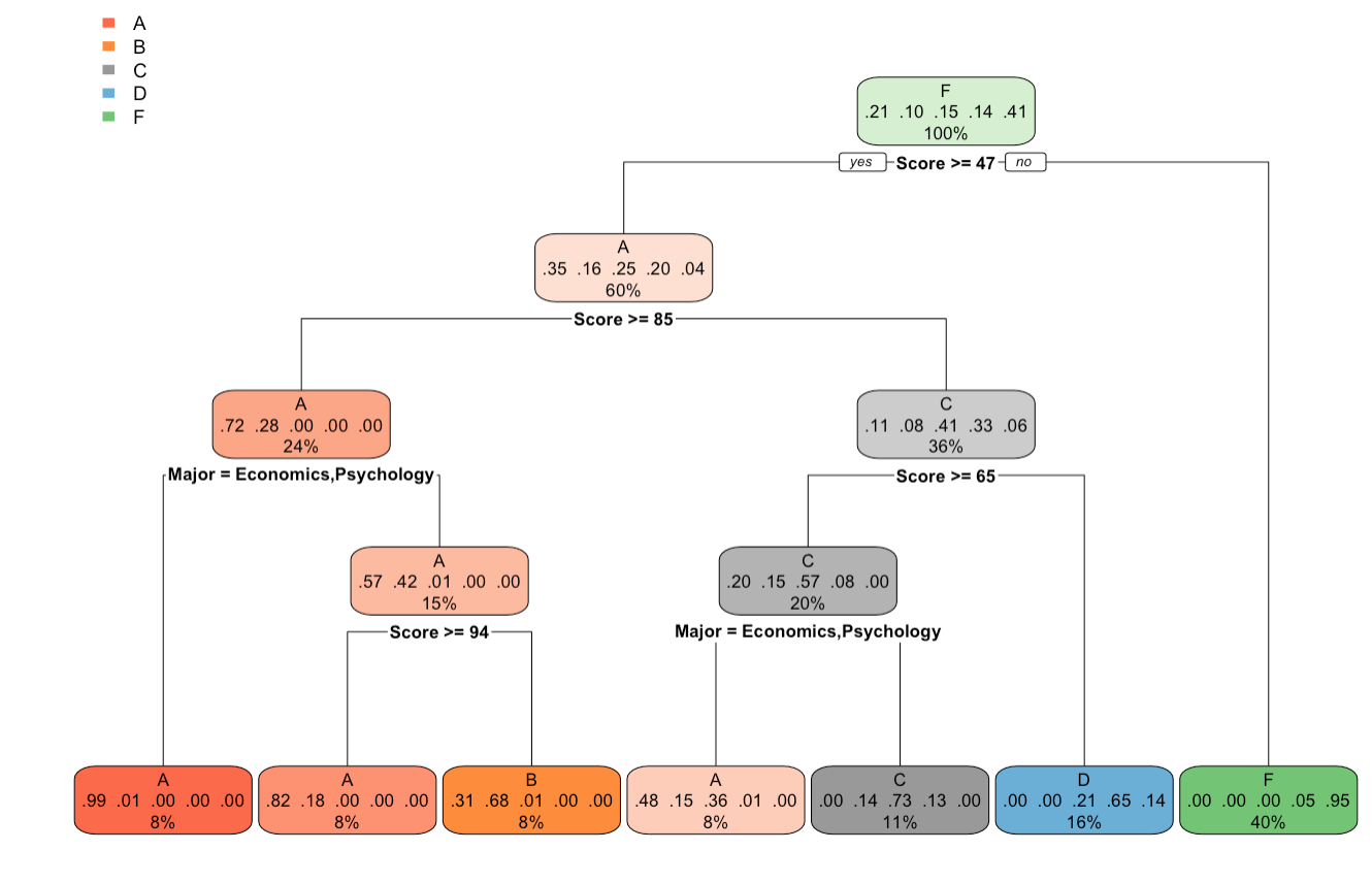
Output Plot of rpart.plot() function
We can see that after plotting the tree using rpart.plot() function, the tree is more readable and provides better information about the splitting conditions, and the probability of outcomes. Each leaf node has information about
- the grade category.
- the outcome probability of each grade category.
- the records percentage out of total records.
To study more in detail the arguments that can be passed to the rpart.plot() function, please look at these guides rpart.plot and Plotting with rpart.plot (PDF)
| NOTE: In this chapter, from this point forward, the rpart.plots() generated in any example below will be shown as images, and also the code to generate those rpart.plots will be commented in the interactive code blocks. If you want to generate these plots yourself, please use a local Rstudio or R environment. |
17.4 Rpart Control
Now let’s look at the rpart.control() function used to pass the control parameters to the control argument of the rpart() function.
rpart.control( *minsplit*, *minbucket*, *cp*,...)- minsplit: the minimum number of observations that must exist in a node in order for a split to be attempted. For example, minsplit=500 -> the minimum number of observations in a node must be 500 or up, in order to perform the split at the testing condition.
- minbucket: minimum number of observations in any terminal(leaf) node. For example, minbucket=500 -> the minimum number of observation in the terminal/leaf node of the trees must be 500 or above.
- cp: complexity parameter. Using this informs the program that any split which does not increase the accuracy of the fit by cp, will not be made in the tree.
For more information of the other arguments of the rpart.control() function visit rpart.control
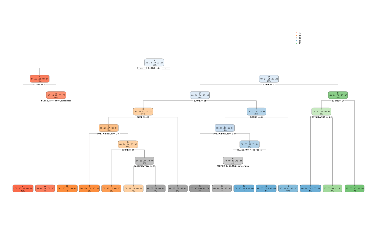
Let look at few examples.
Suppose you want to set the control parameter minsplit=200.
17.4.1 rpart(): Minsplit = 200
Output tree plot of after setting minsplit=200 in rpart.control() function
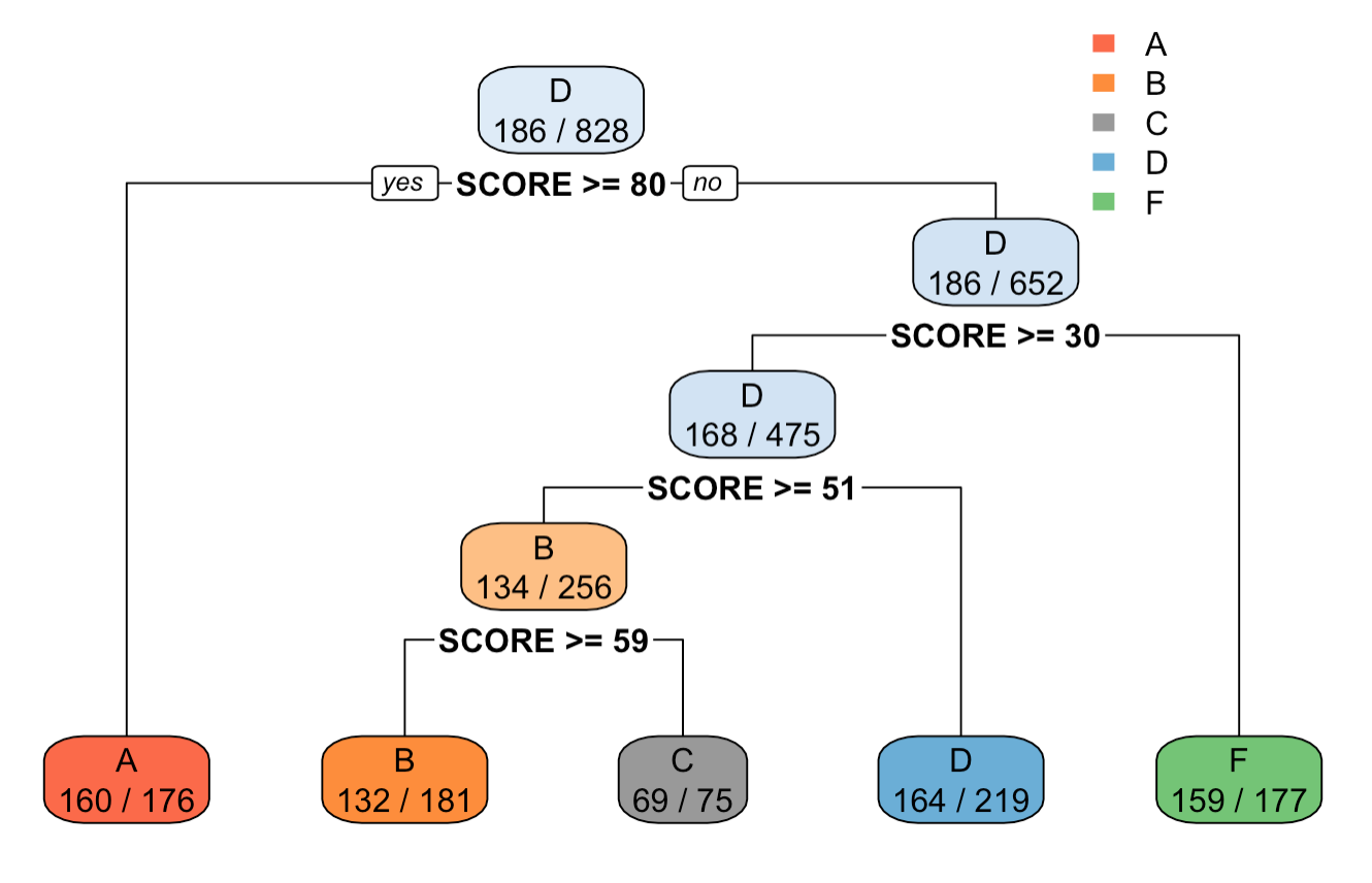
17.4.2 rpart(): Minsplit = 100
Output tree plot of after setting minsplit=100 in rpart.control() function
We can see from the output of tree$splits and the tree plot, that at each split the total amount of observations are above 200 and 100. Also, in comparison to the tree without control, the tree with control has lower height, and lesser count of splits.
Now, lets set the minbucket parameter to 100, and see how that affects the tree parameters.
17.4.3 rpart(): Minbucket = 100
Output tree plot of after setting minbucket=100 in rpart.control() function
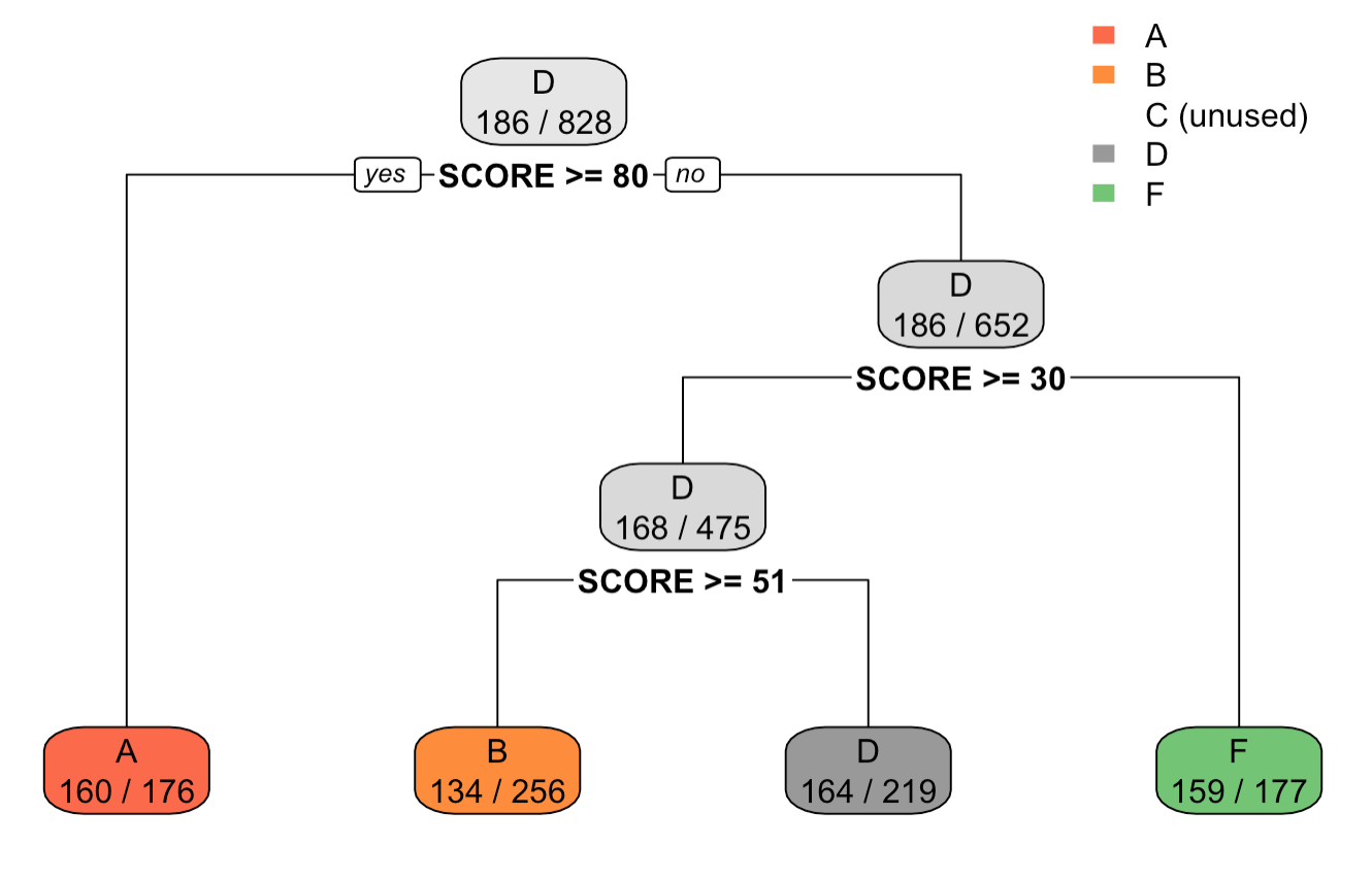
We can see for the output and the tree plot, that the count of observations in each leaf node is greater than 100. Also, the tree height has shortened, suggesting that the control method was able to shorten the tree size.
17.4.4 rpart(): Minbucket = 200
Output tree plot of after setting minbucket=200 in rpart.control() function
We can see for the output and the tree plot, that the count of observations in each leaf node is greater than 200. Also, the tree height has shortened, suggesting that the control method was able to shorten the tree size.
Lets now use the cp parameter and see its effect on the tree.
17.4.5 rpart(): cp = 0.05
Output tree plot of after setting cp=0.05 in rpart.control() function
17.4.6 rpart(): cp = 0.005
 We can see for the output and the tree plot, that the tree size has increased, with increase in number of splits, and leaf nodes. Also we can see that the minimum CP value in the output is 0.005.
17.5 Cross Validation
Overfitting takes place when you have a high accuracy on training dataset, but a low accuracy on the test dataset. But how do you know whether you are overfitting or not? Especially since you cannot determine accuracy on the test dataset? That is where cross-validation comes into play.
Because we cannot determine accuracy on test dataset, we partition our training dataset into train and validation (testing). We train our model (rpart or lm) on train partition and test on the validation partition. The partition is defined by split ratio. If split ratio =0.7, 70% of the training dataset will be used for the actual training of your model (rpart or lm), and 30 % will be used for validation (or testing). The accuracy of this validation data is called cross-validation accuracy.
To know if you are overfitting or not, compare the training accuracy with the cross-validation accuracy. If your training accuracy is high, and cross-validation accuracy is low, that means you are overfitting.
cross_validate(*data*, *tree*, *n_iter*, *split_ratio*, *method*)- data: The dataset on which cross validation is to be performed.
- tree: The decision tree generated using rpart.
- n_iter: Number of iterations.
- split_ratio: The splitting ratio of the data into train data and validation data.
- method: Method of the prediction. “class” for classification.
The way the function works is as follows:
- It randomly partitions your data into training and validation.
- It then constructs the following two decision trees on training partition:
- The tree that you pass to the function.
- The tree is constructed on all attributes as predictors and with no control parameters. -It then determines the accuracy of the two trees on validation partition and returns you the accuracy values for both the trees.
The values in the first column(accuracy_subset) returned by cross-validation function are more important when it comes to detecting overfitting. If these values are much lower than the training accuracy you get, that means you are overfitting.
We would also want the values in accuracy_subset to be close to each other (in other words, have low variance). If the values are quite different from each other, that means your model (or tree) has a high variance which is not desired.
The second column(accuracy_all) tells you what happens if you construct a tree based on all attributes. If these values are larger than accuracy_subset, that means you are probably leaving out attributes from your tree that are relevant.
Each iteration of cross-validation creates a different random partition of train and validation, and so you have possibly different accuracy values for every iteration.
Let’s look at the cross_validate() function in action in the example below.
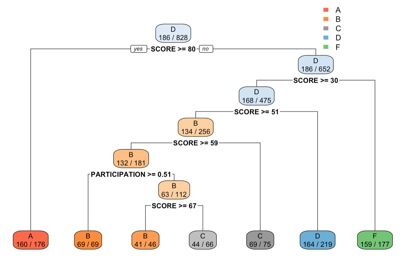
We will pass the tree with formula as GRADE ~ SCORE+DOZES_OFF+TEXTING_IN_CLASS+PARTICIPATION, and control parameter, with minsplit=100.
And for cross_validate() function, we will usen_iter=5, and split_raitio=0.7
| NOTE: Cross-Validation repository is already preloaded for the following interactive code block. Thus you can directly use the cross_validate() function in the following interactive code block. But if you wish to use the code_validate() function locally, please use |
install.packages("devtools")
devtools::install_github("devanshagr/CrossValidation")
CrossValidation::cross_validate()
17.5.1 cross_validate()
You can see that the cross-validation accuracies for the tree that was passed (accuracy_subset) are fairly high and close to our training accuracy of 84%. This means we are not overfitting. Also observe that accuracy_subset and accuracy_all have the same values, which means that the only relevant attributes are score and participation, and adding more attributes doesn’t make any difference to the tree. Finally, the values in accuracy_subset are reasonably close to each other, which mean low variance.
17.6 Prediction using rpart.
Now that we have seen the process to create a decision tree and also plot it, we will like to use the output tree to predict the required attribute.
From the moody example, we are trying to predict the grade of students. Lets look at the predict() function to predict the outcomes.
predict(*object*,*data*,*type*,...)- object: the generated tree from the rpart function.
- data: the data on which the prediction is to be performed.
- type: the type of prediction required. One of “vector”, “prob”, “class” or “matrix”.
Now lets use the predict function to predict the grades of students using the tree generated on the Moody dataset.
17.6.1 predict()
17.7 Combining multiple prediction models
How to build highly predictive models?
This is the million dollar question which many students always ask in the context of our Prediction Challenges (see the leaderboard for 2022). These usually consist of 4-5 prediction tasks and students who achieve the lowest cumulative error make it to the top of the leaderboard and are widely celebrated. What is the secret of building a competitive prediction model? It is not blind application of machine learning library functions such as rpart(). Even with the great set up of parameter values and careful cross validation a singular model will usually not be very competitive. The top prediction models combine human ingenuity, knowledge of data with machine learning library functions. But how to combine different prediction models to build the “supermodel”:-)? . First - know your data, do some preliminary freestyle data exploration, make some plots, see how data is distributed. Possibly identify subsets of data which may behave very differently and may require different prediction models - either “hand made” or ML made.
We will start by showing how to combine two different prediction models - applied to different partitions of the data set. We assume that the partition is “given”. It is usually the result of preliminary data exploration and plotting. In the next section we show an elegant and generic method of combining arbitrary numbers of prediction models using rpart() function.
For now, let us assume that we have partitioned the moody data set based on the attribute SCORE into two subsets: one with SCORE >50 and another with SCORE <=50. Furthermore we have trained separate rpart() prediction models for each of the two partitions. Now we want to combine these two models into the one, combined model and apply the combined model to the testing data set moodyTest.
The following snippet 16.6.1 shows how to do it. Two models: model1 and model2 are trained by running rpart() on two partitions of moody - *the training data set, based on SCORE. Then we use predict() function by applying model1 to the partition of SCORE >50 and model2 for the subset defined by SCORE <=50 of the testing data set - moodyTest. Finally the lines 11-14 built the decision vector which combines predictions of models 1 and 2 into one prediction vector on the moodyTest.
17.7.1 Combining rpart prediction models
17.7.2 Combining multiple prediction models using rpart
We describe here an elegant method which will allow us to build a combined model in two (or more) phases. Let us start with two prediction models: pred1 which is freestyle model and pred2 which is rpart() model. We have faced this situation in our prediction challenges in the spring of 2022. Students were asked to create two prediction modes: one, which was their own code (freestyle prediction) and another - through application of rpart(). Turned out that top freestyle prediction models had lower error on the testing data than rpart(). The challenging task was to combine two models and make the best out of the two, hopefully getting a combined model which beats both freestyle and rpart() models. But how to build such a model? In the previous section we just described the mechanics of combining two models - by splitting the data set into two disjoint partitions and applying each model to just one partition. But how to find such partitions? Fortunately we have rpart() to help us.
We will demonstrate the proposed method using some pseudo-code and then illustrate it further with an executable snippet combining two specific prediction models. We will expand first the training (and testing) data with two additional, derived attributes. One for each prediction model. Call these attributes \(model1\) and \(model2\). Then use rpart() to find the best model which uses original attributes of the data set as well as these two new attributes. Therefore we just let rpart() decide what is the best use of these two new attributes.
Let df_train be the training data set (data frame) and let df_test be the testing data frame. Let pred_yourModel be the freestyle prediction function which returns a decision vector according to a freestyle prediction model. For example 16.6.2 snippet shows such a very simplistic model for a moody data set, which assigns grades based on the disjoint intervals of SCORE attribute.
df_train$model1<- pred_yourModel(df_train)
tree<-rpart(df_traing,...)
df_train$model2 <- predict(tree, test, type="class")

Now, the training data set has two extra attributes: model1 and model2.

Finally we create a compound model by using the extended attribute set of moody.

Tree_combined <- rpart(F, data = df_train, method = "class"))

F is of the form T~.  where T is the target attribute of df (the one we predict). We let rpart() use all attributes including the new ones: model1 and model2.

Tree_combined will use both prediction models as attributes and depending on their information gain these two new attributes may play an important role. We can cross validate like before and estimate the error of this combined prediction model on the training data set.

If we are satisfied with the combined model, we then repeat the same process on testing data.

df_test$model1<- pred_yourModel(df_test)
tree<-rpart()
df_test$model2 <- predict(tree, df_test, type="class")
Now, the training data set has two extra attributes: model1 and model2.

And calculate final prediction using predict function:

predict(Tree_combined, moody_test, type="class")


The next snippet illustrates this process  for a moody data set.  Freestyle model is very simplistic:

decision <- rep('F',nrow(moody))
decision[moody$Score>40] <- 'D'
decision[moody$Score>60] <- 'C'
decision[moody$Score>70] <- 'B'
decision[moody$Score>80] <- 'A'
moody$model2 <-decision
This prediction model assigns grades solely on the basis of SCORE attribute: A’s for SCORE over 80, B’s for SCORE between 70 and 80, C’s for SCORE between 60 and 70, D’ s for SCORE between 40 and 60 and finally F for SCORE <40.
We combine this model with model1 which uses rpart().
Last two lines of the code show where model1 and model2 differ and how often do these two models differ (in almost 25% of the data set)
17.7.2.1 Combining two prediction models using rpart() for moody data set
| SCORE | GRADE | DOZES_OFF | TEXTING_IN_CLASS | PARTICIPATION | model1 | model2 | |
|---|---|---|---|---|---|---|---|
| 758 | 69.03 | B | never | never | 0.60 | B | C |
| 156 | 46.93 | C | sometimes | rarely | 0.03 | C | D |
| 364 | 34.50 | F | sometimes | rarely | 0.47 | D | F |
| 753 | 46.07 | C | sometimes | rarely | 0.83 | C | D |
| 183 | 58.99 | C | sometimes | never | 0.29 | C | D |
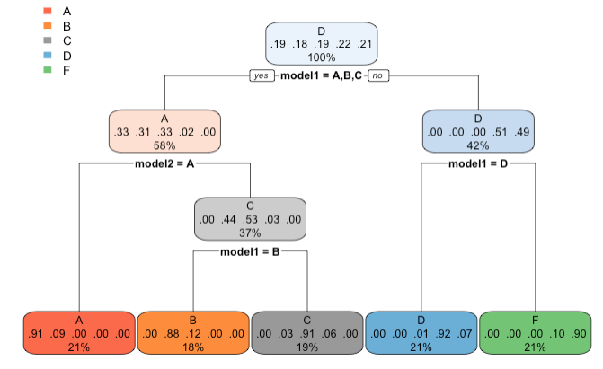
Output tree plot of after combining model1 and model2
Next snippet shows how to submit your prediction vector to Kaggle by creating your submission data frame.