Section: 2 Setting Up R
Important Instructions
- Installation of R is required before installing RStudio
- “R” is a programming language, and,
- “RStudio” is an Integrated Development Environment (IDE) which provides you a platform to code in R.
- Installation of R is required before installing RStudio
How to download and install R & RStudio?
Downloading and installing R.
- For Windows Users.
- Click on the link provided below or copy paste it on your favourite browser and go to the website.
- Click on the link at top left where it says “Download R 4.0.3 for windows” or the latest at the time of your installation.
- Open the downloaded file and follow the instructions as it is.
- For MAC Users.
- Click on the link provided below or copy paste it on your favourite browser and go to the website.
- Under “Latest release”, click on “R-4.0.3.pkg” or the latest at the time of your installation.
- Open the downloaded file and follow the instructions as it is.
- For Windows Users.
Downloading and installing RStudio.
- For Windows Users.
- Click on the link below or copy paste it in your favourite browser.
- Scroll down almost till the end of the web page until you find a section named “All Installers”.
- Click on the download link beside “Windows 10/8/7” to download the windows version of RStudio.
- Install RStudio by clicking on the downloaded file and following the instructions as it is.
- For MAC Users.
- Click on the link below or copy paste it in your favourite browser.
- Scroll down almost till the end of the web page until you find a section named “All Installers”.
- Click on the link beside “macOS 10.13+” to start your download the MAC version of RStudio.
- Install RStudio by clicking on the downloaded file and following the instructions as it is.
- For Windows Users.
2.1 Create New Project
After installing R studio successfully the first step is to create a project R studio.
- Step 1: Go to File -> New Project
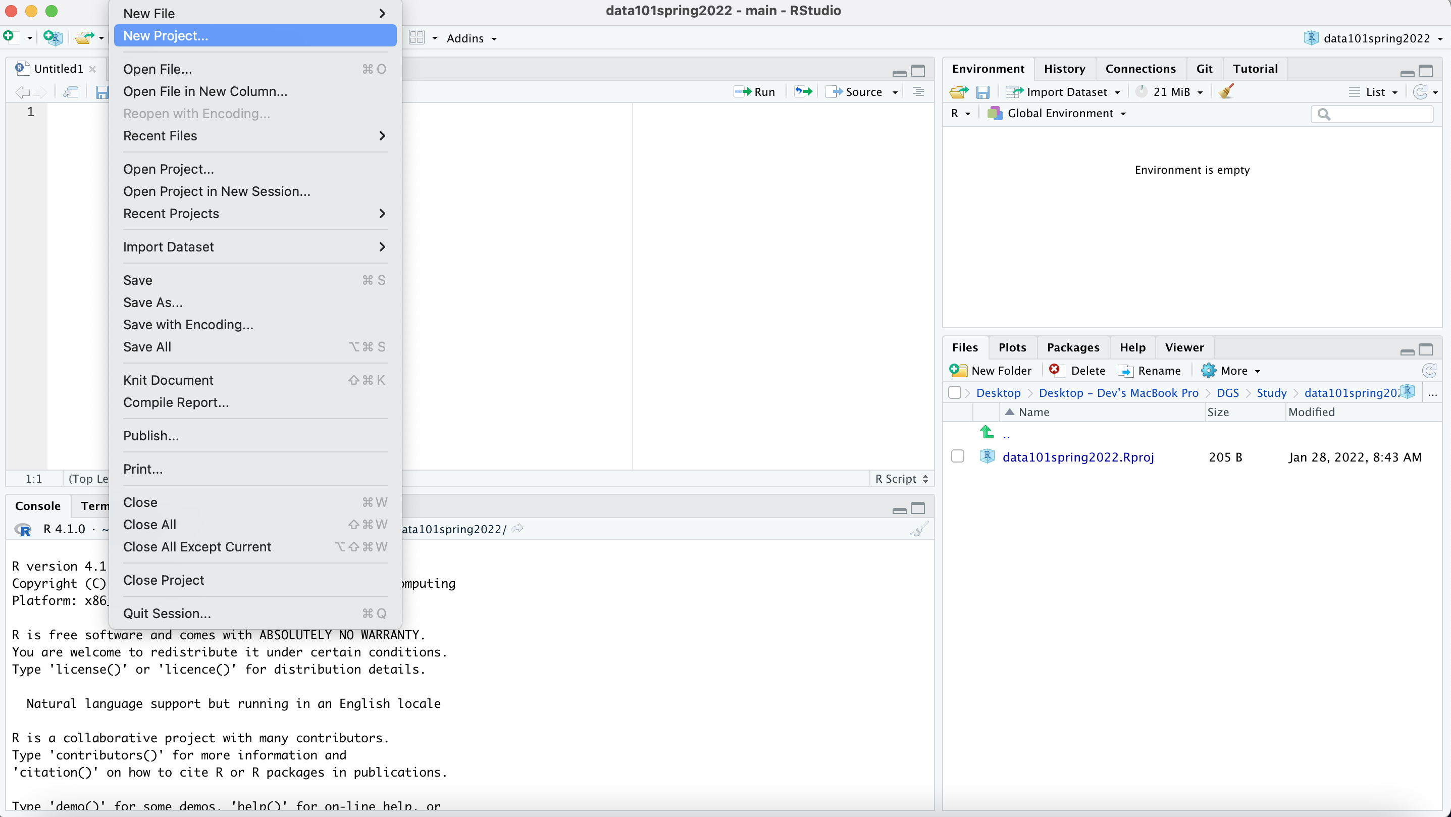
New Project
- Step 2: Select New Directory
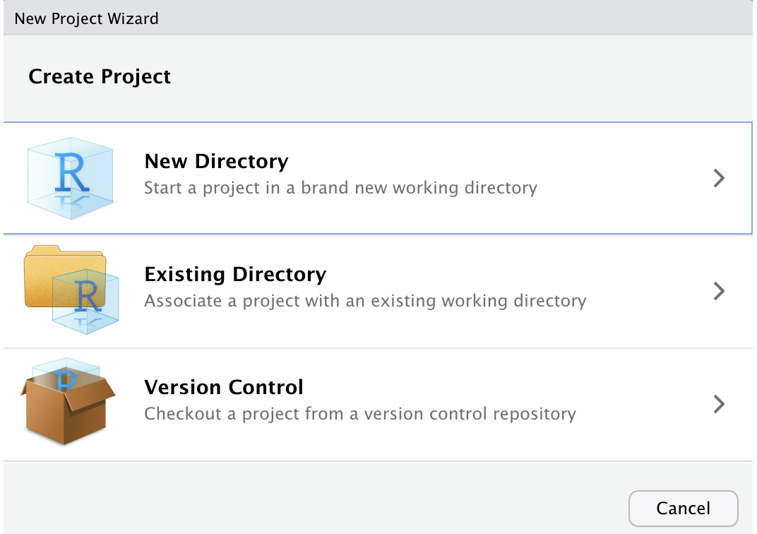
New Directory
- Step 3: Select New Project
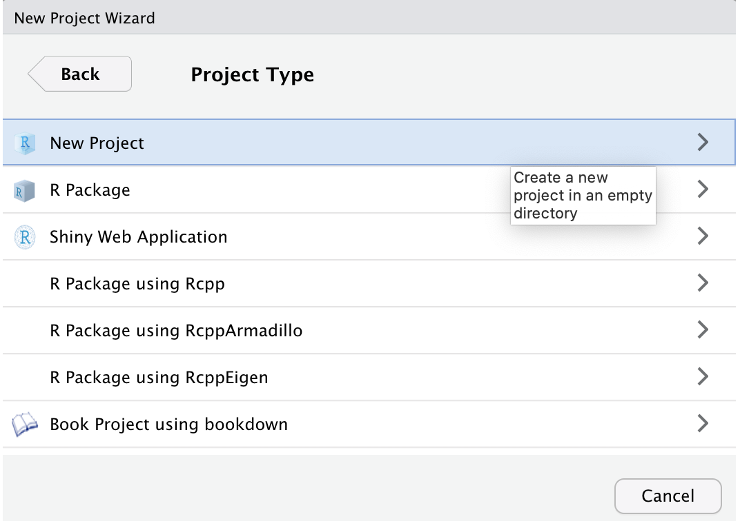
New Project
- Step 4: Give your preferred directory name like “Data101_Assignmnets”
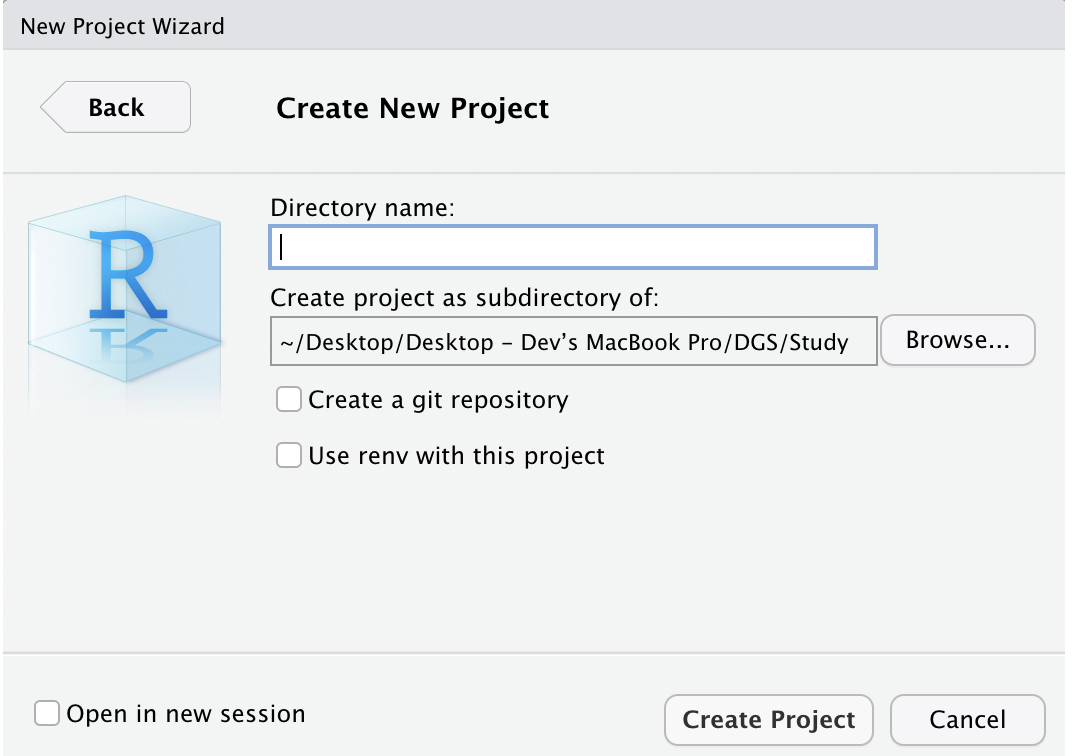
Directory Name
- Step 5: Click on Create Project and finally the R studio should look like
Rstudio
2.2 How to upload a data set?
2.2.1 Grades dataset
Download: moody2022.csv
Grades in Professor Moody’s class data set.
Our working data set will be the Moody data set which stores data about students’ grades in a large signature class taught by Professor Moody. The data set stores individual scores of students in class, their major, seniority and GPA. Data scientists may ask many questions such as, given the student’s score in class, does the final grade depend on the major and/or student’s seniority? For example, is it more difficult for computer science majors to earn an A, pass the class, than, say for students majoring in psychology? Does GPA play any role in grading? It should not - but maybe it does? We are still far away from being able to ask such questions, for now we will use Moody data set in code snippets which illustrates the core R functions which we will use in the active textbook.
| Major | Score | Seniority | GPA | Grade | |
|---|---|---|---|---|---|
| 706 | CS | 69 | Junior | 3 | C |
| 249 | CS | 75 | Junior | 1 | C |
| 855 | Psychology | 68 | Freshman | 4 | C |
| 585 | Statistics | 42 | Senior | 2 | F |
| 705 | Economics | 52 | Sophomore | 4 | D |
To upload the dataset/file present in csv format the read.csv() and read.csv2() functions are frequently used The read.csv() and read.csv2() have different separator symbol: for the former this is a comma, whereas the latter uses a semicolon.
There are two options while accessing the dataset from your local machine:
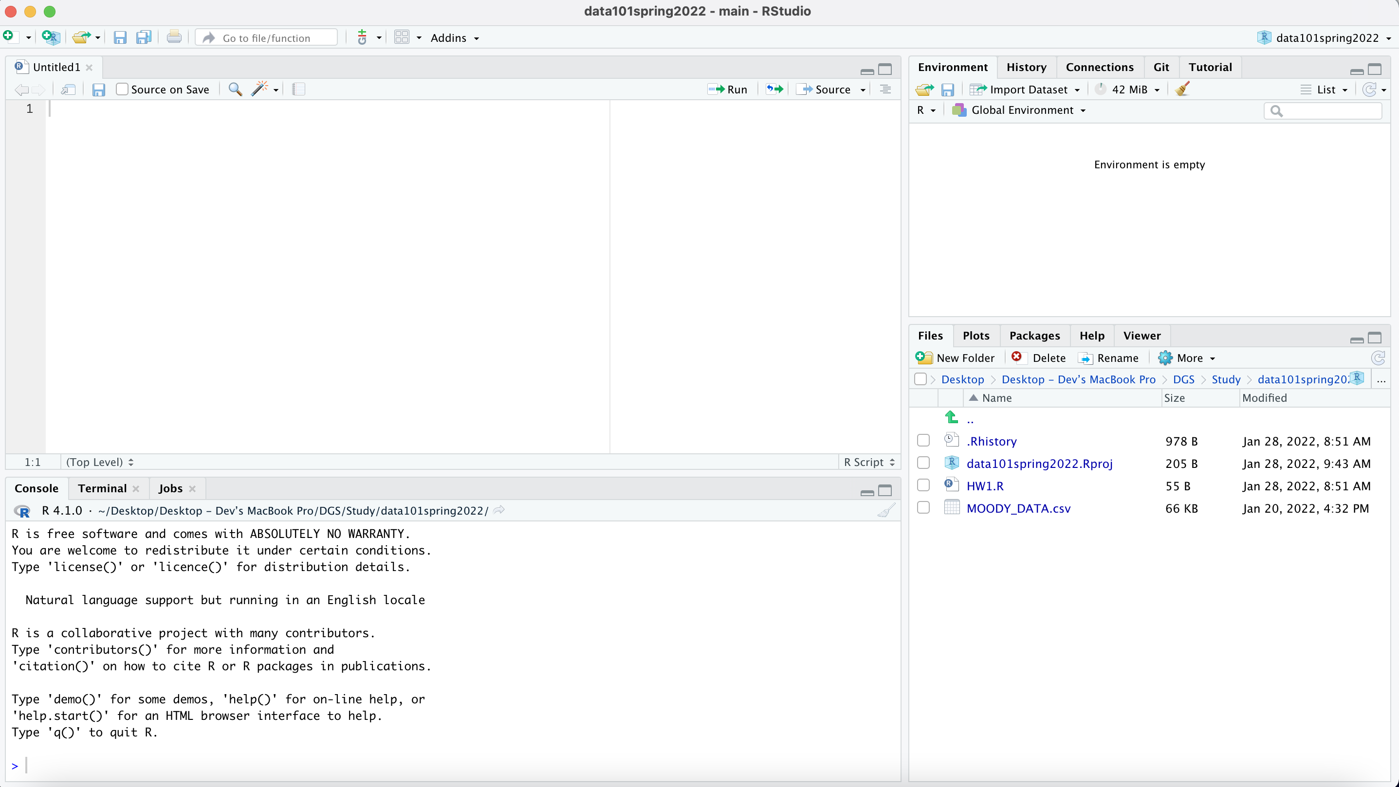
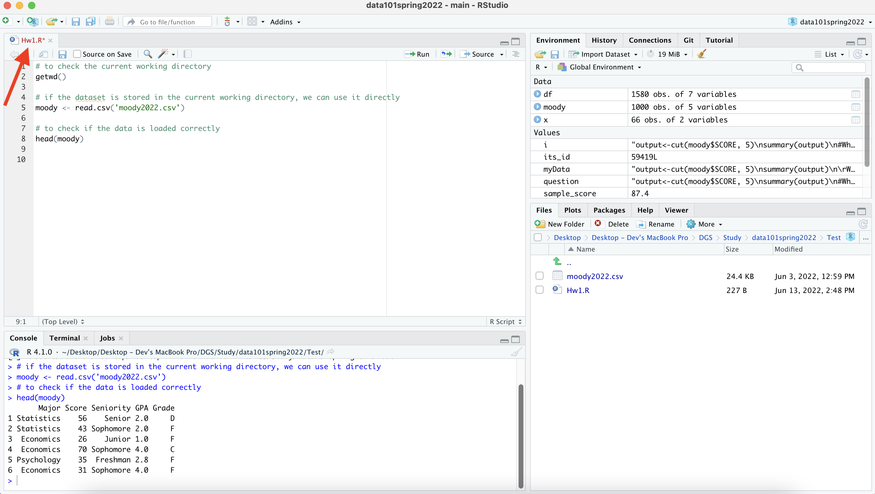
- To avoid giving long directory paths for accessing the dataset, one should use the command getwd() to get the current working directory and store the dataset in the same directory.
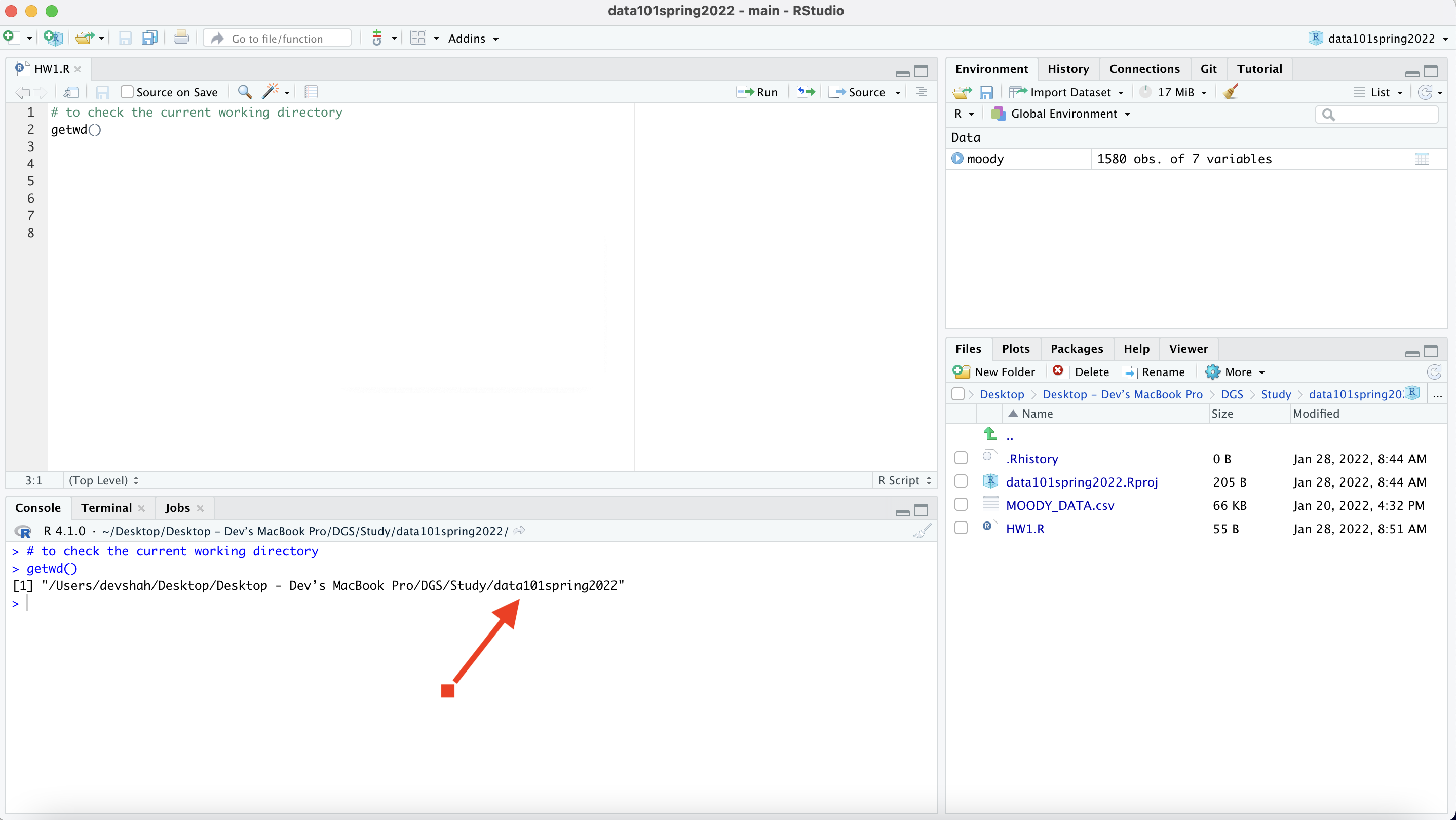
Getwd
- To access the dataset stored in the same directory one can use the following: read.csv(“moody2022.csv”).
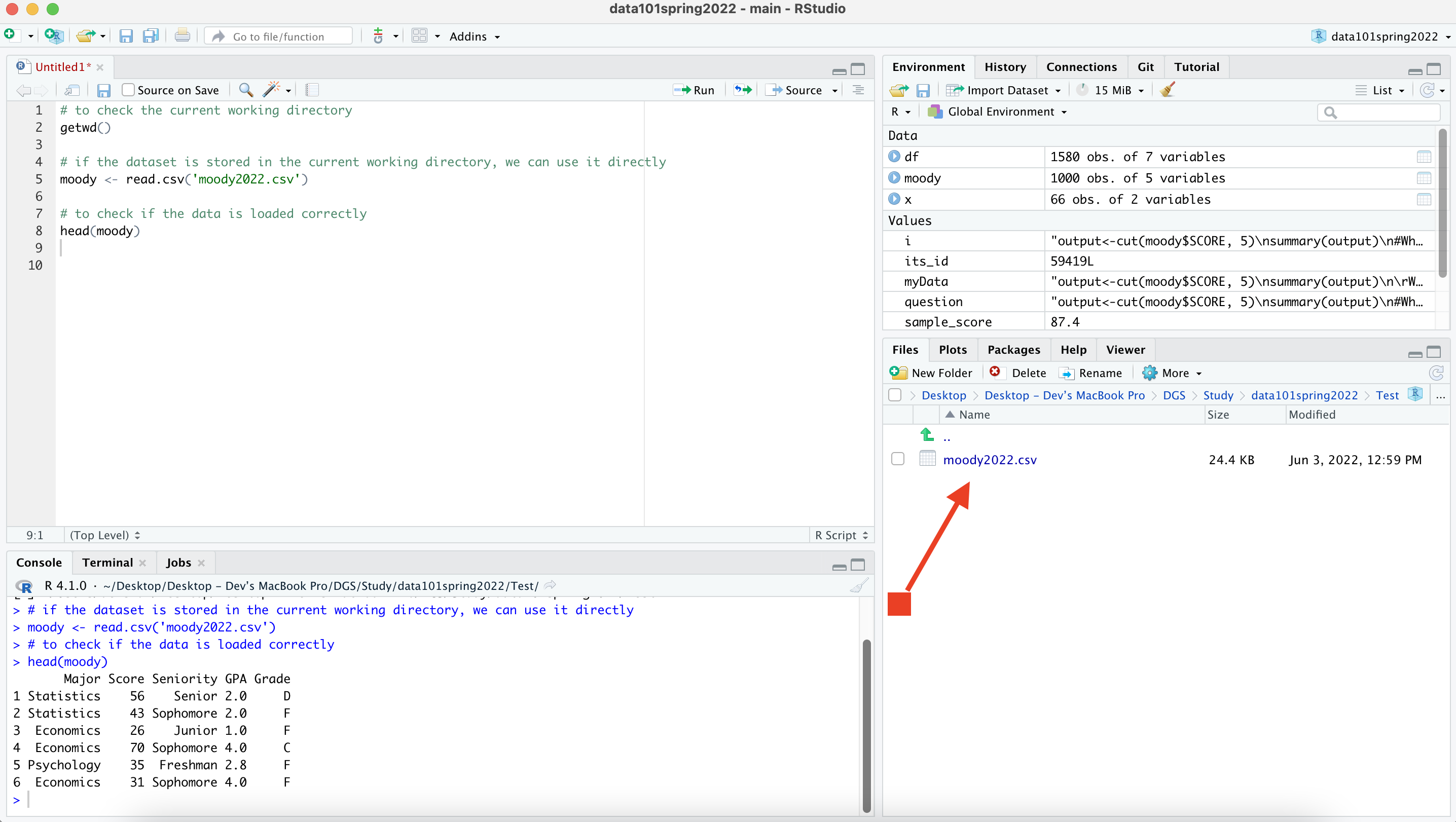
Store the moody dataset in the same directory
- One can also store the dataset at a different location and can access it using the following command: (Suppose the dataset is stored inside the folder Data101_Tutorials on the desktop)
- For Windows Users.
  - Example: read.csv("C:/Users/Desktop/Data101_Tutorials/moody2022.csv")

- For MAC Users.
  - Example: read.csv("/Users/Desktop/Data101_Tutorials/moody2022.csv")
2.3 Saving your work
- To save your work go to File -> Save. It will ask you to give a name for your .R file and then click on Save.
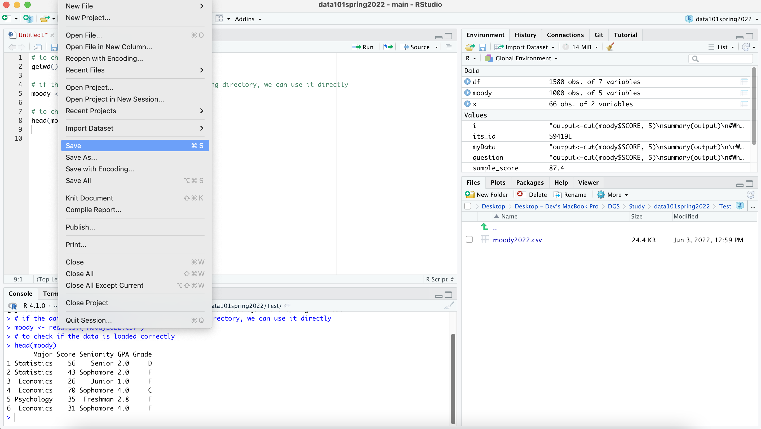
Save
- After making modifications to your saved file, you will need to save the file again. If the name of the file on the top is in Red Color indicates that the file have unsaved changes.
Unsaved File
- Go to File -> Save to save your .R file again. After saving the file the color of the file name i.e. HW1.R will again change back to black.

Saved File
Note: You can create multiple files inside the same project such as for your each homework assignments
2.4 General R References
https://www.w3schools.com/r/
https://cran.r-project.org/doc/contrib/Short-refcard.pdf
https://www.amazon.com/Statistics-Engineers-Scientists-William-Navidi/dp/0073376337/ref=pd_lpo_3?pd_rd_i=0073376337&psc=1
https://data101.cs.rutgers.edu/laboratory/
2.5 Textbook Concepts
Hypothesis testing: 9
Difference of means hypothesis testing: 9
Null Hypothesis: 9
Alternative Hypothesis: 9
z-value: 9
critical value: 9
significance level: 9
p-value: 9
Bonferroni correction: 12
Chi square test: 10
Independence: 10
Multiple Hypothesis testing: 12
False Discovery Proportion: 12
Contingency Matrix: 10
Bayesian Reasoning: 13
Prior odds: 13
Posterior odds: 13
Likelihood ratio: 13
False positive: 13
True positive: 13
Crossvalidation: 17.5
Decision trees: 17
Linear regression: 18
Recursive partitioning: 18
MSE: 18
Prediction accuracy: 18
Training: 18
Testing: 18
2.6 R functions used in this class
Elementary instructions: c() 3.1, mean() 3.4.1, nrow() 3.5.1, rep(), sd() 3.4.5, cut() ??
Plots: plot() 4.1, barplot() 4.2, boxplot() 4.3 mosaicplot() 4.4
Data Transformations: subset() 3.5, tapply() 3.6, table() 3.3, aggregate()
Library functions: chisq.test() 10, pnorm() 9.2, Permutation() 9.2, rpart() 17, predict() 17.6, lm() 18.2, crossvalidation() 17.5