Section: 6 Fooled By Randomness
In this section we show how random data can fool us. Often, random findings may look real, in fact so real that we mistake them for real discoveries. It is one of the main objectives of statistics and data science to help identify such false discoveries. This chapter provides a motivation and justification for hypothesis testing methods, multiple hypothesis corrections, p-values and permutation tests which we discuss in subsequent sections of the active textbook.
Here we show how randomly generated data set can lead to seemingly astonishing discoveries – which are simply …random, although they look anything but random!
In order to illustrate false discoveries we have used our DataMaker data generation tool to generate a data set Cars describing hypothetical sales data for car dealerships in 15 major cities in the US. We have considered 10 major car makers, different seasons of the year (winter, spring, summer, fall). In addition Cars stores information about buyer gender as well as buyer’s age. Below we show a sample of several tuples of Cars
| Dealership | Season | Car | Buyer | Buyer_Age | |
|---|---|---|---|---|---|
| 21149 | LA | Winter | Ford | Female | 63 |
| 41124 | San Diego | Spring | GMC | Female | 41 |
| 44861 | Chicago | Fall | Subaru | Female | 69 |
| 32580 | Austin | Winter | Honda | Female | 44 |
| 29415 | San Antonio | Winter | Honda | Female | 53 |
We have generated the Cars data set as completely random data set, with uniform distributions of dealerships, car makes sold there, four seasons, buyer’s gender’s and their age. Thus any buyer with any age is equally likely to buy any car in any of the dealerships.
We have run several queries on Cars dataset and demonstrated through the following snippets, how random data can lead to query findings which look “real”.
Let us start with the first snippet which shows that indeed our data set follows uniform distribution and it has been randomly generated.
Snippet 6.1: Get to know your dataWe can see that each car maker is sold around 9% of the time, and 9% of transactions take place in each of the dealerships from LA to NYC. We also see that around 25% of transactions take place in each season. Also buyers’ gender is distributed equally 50:50 across all transactions for each car and for each dealership. In other words, nothing interesting is happening in this data – it is unrealistically uniform.
Nevertheless, even this purely random data leads to some seemingly exciting discoveries. We will first show a few examples of these false discoveries and then follow up with explanations how such discoveries can emerge out of pure randomness. How can we be so fooled and what are remedies to avoid trusting such random discoveries?. In the second subsection we discuss sampling and dangers which emerge from drawing conclusions from data samples.
6.1 False Discoveries
Here we list some of the false discoveries:
Snippet 6.2: Among very young customers (Age <22) of Chicago dealership Dealership, 12.2% buy Hyundai and only 7.4% by GMC. Thus, almost twice as many of the very young customers prefer Hyundai to GMC.
Snippet 6.3: Among senior customers (Age >70) of LA dealership, 13.1% buy Toyota and only 6.25% buy GMC. Interesting findings! Twice as many seniors in LA buy Toyota than GMC!
Snippet 6.4: Gender distribution of Honda purchases in Austin dealership favors female customers – 54% Female to 46% Male
We discover seemingly a significant disparity between genders among Honda Buyers in Austin. 8% difference between female and male customer share seems significant.
Snippet 6.5: Mean age of Jeep buyers in Chicago in spring is 4 years higher than in summer. It is 54 in spring vs 50 in spring.
Younger Jeep Buyers in Chicago wait for summer!
Snippet 6.6: The gender gap among GMC buyers in LA who are in late twenties is 22%!, 61% are female and only 39% are Male
GMCs are drastically more popular among women than among men in LA. Certainly all these discoveries are false! Tricks that random data plays on us.
There is a number of factors leading to these false discoveries:
Subsets of data are pretty narrow – GMC buyers in winter in one dealership who are in a certain age bracket constitute a small subpopulation of the whole data set. So called Law of small numbers which we discuss later states that such small data sets are prone to extreme results.
There is an exponential number of queries which look like 6.1-6.5 and differ only by choice of parameters (age, dealership name, and car make name). Running a sufficient number of such queries every time changing one or more parameters, we are simply bound to find some false positives. This is called multiple hypothesis testing. Before we presented queries 6.1-6.5 above we have run a number of queries which did not generate false discoveries. This is sometimes called p-value hunt and multiple hypothesis testing and Bonferroni coefficient (discussed in section 9) takes this trial and error process under consideration.
Difference of means may be due to a simple random process. We need a permutation test, z-test and similar test to see if a conclusion like 6.3 is statistically legitimate. It is not. But we cannot just eyeball it and decide.
6.2 More about Sampling
We have already shown the distribution of prices of Brooklyn apartments across samples of different sizes. Here we show more examples of sampling and its impact on different queries.
We will begin by showing how we select a sample of a given size from the data set. Here for Cars, we select 5000 random tuples from the total of 50,000 tuples.
Snippet 6.7: Sampling
The function sample() permutes the rows of Cars data frame. Then we select the first 5000 tuples from the shuffled Cars data frame (you may change this number).
Now let us run several queries on the samples and compare them with the results of the same queries over the entire Cars data set. Note: students are encouraged to run sampling code multiple times and see how query results change! This should serve as a warning about trusting samples. One can also change the sample size and see what effect does it have on a query.
Snippet 6.8: Effect of random samples of different sizes on the average age of a buyer.
Snippet 6.9: Effect of random samples of different sizes on the average age of a buyer of Ford in Chicago
The more narrow is the query, the more discrepancy there is between query results over samples.
Snippet 6.10: Skewed car maker distributions among female buyers older than 45 in theSan Antonio dealership
We observe a very skewed result here – Honda is best seller among Female buyers over 45 in San Antonio, with 14% buyers of Honda vs just 5.4% buyers of GMC.
We have generated three more samples and every time the best seller in this group of buyers was different!
- First Sample:
- Jeep 14.5% (bestseller)
- Nissan 4.8% (worst seller) - The gap of almost 10%!
- Second Sample:
- Huyndai 11.8%
- Jeep 5.2%
- Third Sample:
- GMC (11.8%)
- Chevrolet (4.7%)
Quite a variation!
Let us now take one specific Car make-, say GMC and analyze its purchases among buyers younger than 30
Snippet 6.11: Analysis of market for GMC buyers
We can observe quite substantial variation of GMC market share among buyers younger than 30. The market share varies from 6 to 10% among different samples. In general samples become more sensitive also with more narrow queries. If we only considered GMC market share (dropping age constraints), we would observe much smaller market share variation.
Snippet 6.12 Average age distribution grouped by all car makes in in Chicago
Notice how for a smaller sample of 500 the distribution of average age varies for different car makes – from almost 60 for Subaru to around 40 for Nissan.
6.3 Confidence Intervals
| Party | VoterID | |
|---|---|---|
| 2153 | Democratic | 12084 |
| 12709 | Republican | 18759 |
| 5794 | Republican | 10302 |
| 2018 | Democratic | 9342 |
| 14387 | Democratic | 6720 |
This data contains synthetic data on 200000 voters in some small county who voted either Democrat or Republican. The majority of voters (55%) voted republican, while the minority voted for Democrats. Typically votes are not counted simultaneously and we are all familiar with “calling elections” on the basis of a smaller subset of counted votes.
In the following snippet we would like students to experience the effects of samples of different sizes. Samples may provide different results from an even more decisive win of Republicans (like 60%+) to a slight win by Democrats.
Snippet 6.13: Distribution of votes for Democrats vs Republicans in a random sample of 100 voters may deviate from 45:55 split in the general population.
Just run the code several times and observe how the distribution of votes between Democrats and Republicans changes. Also, change the size of the sample from 100 to 1000 and perhaps even to 10000. Observe how more “stable” the results are and how much closer the vote distribution is now to the true vote distribution in the general population of voters.
The next snippet is the only one when we use a simple for loop in this entire textbook.
Below we display the histogram of 1000 samples of size 500 and we observe how the support for Democrats varies. Please observe that the histogram’s shape approached Bell’s curve with the mean of 45% (true voter support for Democrats). Notice however that there is a fraction of samples which would incorrectly have Democrats as winners, exceeding 50% of vote.
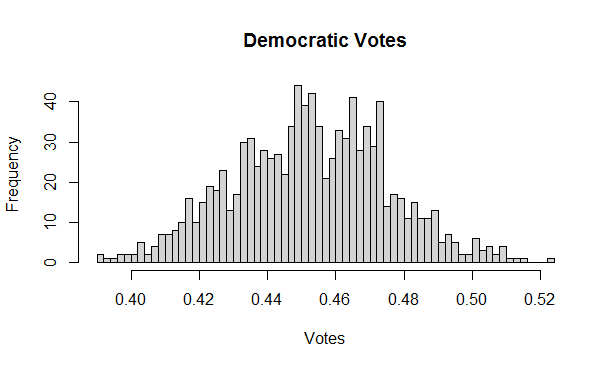
Figure 6.1 Democratic votes
6.4 Law of Small Numbers
The term “Law of small numbers” has been coined by Kahneman in his book “Thinking fast, Thinking slow”.
The law of small numbers states that small samples are more prone to extreme results than large samples. Kahneman refers to the example of incidences of kidney cancers. It seems that kidney cancers are less frequent in small rural counties in mid-west. - probably because life in small rural counties is more healthy, food is organic etc. Unfortunately, kidney cancers are also more frequent in small rural counties in midwest. This time (false) narrative can attribute it to poverty and poor access to healthcare. In fact none of the two narratives is correct. Small samples (small counties in this case) are simply more prone to extreme results. This is analogous to selecting a small number of balls from an urn containing red and black balls. With a small number of balls (4) the extreme results (4 black, 0 red, 4 red, 0 black) occur more often than when the number of selected balls is larger, say 7.
Here we illustrate the law of small numbers using our Car dealerships data set. For small sizes of samples (10), we observe that Winter is the season when car sales are dramatically higher than expected seasonal sales (about 25% of sales for each of the 4 seasons in our synthetic data set). For different samples of size 10, we may conclude that winter is the season when sales are much lower than expected. Thus, the opposite effect!
Use the snippet by running the code several times and also changing the size of the sample from 10 to 20, 30 and down to 5 as well to observe effects of law of small numbers.
Snippet 6.14 Law of small numbers snippet
6.5 Randomness and repeatability
When data is random, “observed” trends do not repeat themselves.. They come and go, with different random samples.
How likely is it that GMC are bought more often by females than males in Columbus, season after season, sample after sample?
If the data is always random, i.e. the next data is again randomly generated, we are likely to see the reversal of the trend. In fact every time we get the new data, data may be reversed. In data science we are looking for lasting trends, we would like to treat the data as representative of the general trend which outlasts the current sample. The whole data set after all is a sample of some unknown “universal data set”. Here we demonstrate what happens when universal data set is in fact randomly uniform,
Notice that if we generate new samples, we may get a complete reversal of the trends, in the same dealership we may get Toyota as most popular and Honda as least popular, and for another sample Toyota and Honda may switch places!
Randomness is the main force fooling us and has to be treated very seriously. Eliminating randomness as the “cause” of our observations is one of the main goals of data science. Hypothesis testing allows us to take randomness into account and the concept of p-value is a quantitative measure of possible impact of random data.
6.6 Data sets with embedded patterns
Using the DataMaker tool we have embedded the following two patterns into Cars data:
Subaru in Austin is bought by 95% females
GMC in Columbus is bought by 93% males
The following snippet shows the skewed distribution of females and males due to the pattern injected by DataMaker into the cars data set.
Snippet 6.15 Car data set with embedded pattern
These two patterns are intended to be legitimate - not false discoveries. We have made them rather extreme, skewing the gender distribution in both cases above 90%. But what if we made it slightly more than the uniform – random distribution in Cars, for example 60:40 distribution? The challenge for statistical evaluation methods is not to reject such True discoveries. The closer the real pattern is through to the possible random pattern, the more likely such False Negatives are. Thus, in the process of rejection of False Positives we may also fall into the trap of False Negatives and reject the legitimate discoveries. Being too cautious may deprive us from discovering a real business value in our data. Being too adventurous, may result in false discoveries. There is a cost associated with each of these two errors. Is it better to be too optimistic than to be too pessimistic?