Section: 19 Power Law Distribution
Power law distributions have been known for a while but came to prominence with the advent of the world wide web where power law occurs quite frequently.
Naseem Taleeb in his book Black Swan has termed Power Law as Extremistan and Normal (Gaussian) distribution as Mediocristan. The Mandelbrotian and the Gaussian. from Mandelbrodt and his pioneering work in the field of fractals and power distribution.
Figure 1 displays power law which reflects acute concentration and so-called long tail characteristics to virtual quantities such as web traffic, sales data, wealth data, youtube views, word frequency etc. Gausian law (Bell curve) usually displays more physical quantities such as weight, height etc. The latter concentrate heavily around mean and decline quickly (so called Gausian decline). Long tail of power law distributions declines much slower and as we will see helps to explain much more wild deviation of wealth, sales etc.

Figure 19.1 Power Law
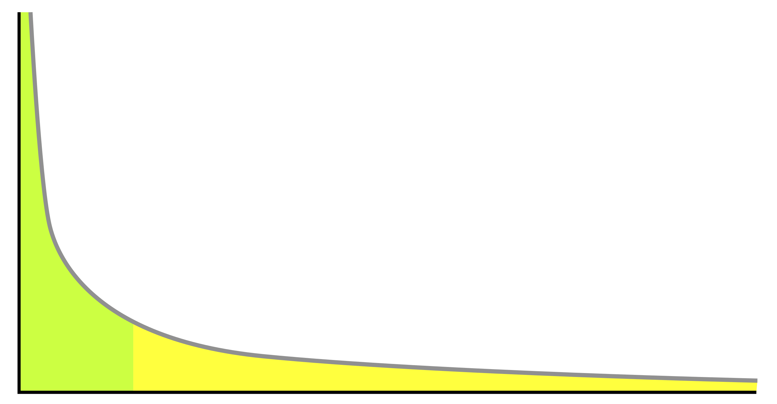
Figure 19.2 Bell curve – Gaussian Distribution
For example, take the height of men and women. Average height is 1.67 meters. It is distributed normally around this mean height. Assume that standard deviation of height is 10 cm.
Consider odds of being
| 10 centimeters taller than the average (i.e., taller than 1.77 m, | 1 in 6.3 |
| 20 centimeters taller than the average (i.e., taller than 1.87 m, or 6 feet 2 | 1 in 44 |
| 30 centimeters taller than the average (i.e., taller than 1.97 m, or 6 feet 6): 1 in 740 | 1 in 740 |
| 40 centimeters taller than the average (i.e., taller than 2.07 m, or 6 feet | 1 in 32000 |
| 50 centimeters taller than the average (i.e., taller than 2.17 m, or 7 feet | 1 in 3,500,000 |
|
60 centimeters taller than the average (i.e., taller than 2.27 m, or 7 feet 70 centimeters taller than the average (i.e., taller than 2.37 m, or 8 feet 9 |
1 in 1,000,000,0000 |
| 100 centimeters taller than the average (i.e., taller than 2.67 m, or 8 feet 9 | 1 in 130,000,000,000,000,000,000,000 |
\[\begin{equation} P(X>x) = a * x ^{-c} \end{equation}\]
Thus if one doubles x (the threshold) then the probability of exceeding x goes down \(2^{-c}\) times. If exponent c=1, then x doubles the \(P(X>2x) = ½ * P(X>x)\)
The following snippet illustrates the radical differences between power law distribution and the normal distribution.
We first generate the power law distribution with the exponent -1. To this aim we first generate uniform distribution (runif() function does this) of real numbers between 0.001 and 1. We are also rounding these numbers up to 3 digits using round(). Power distribution is generated by one line of code
\[\begin{equation} Power < -v ^ {-1} \end{equation}\]
We generate 10000 data points which range from 1000 down to 1. The mean value of the power law distribution is 7. Now to compare the power law distribution and normal distributions we use rnorm() to create 10000 data points distributed normally around the same mean =7 and with standard deviation of 0.1. We show histograms of both distributions to illustrate the different shapes, long tail shape of the power law distribution and the characteristic Bell curve of the Gaussian distribution. Then we follow by illustrating the main point: the rapid descending of the Gaussian distribution. Just change the values in two last statements of the snippet: length(normal[normal>7.1]) and length(power[power>7.1]). Notice that the number of values which are larger than 7.1 (one standard deviation from the mean) is roughly the same for both distributions: it is around 1500. But now observe what happens when we move x higher in length(normal[normal>x]), and length(power[power>x]). The value of x=7.3 is the largest value when there are still 19 values left in length(normal[normal>x]), when we move x to 7.4, this number is already zero. Now compare it with the power law distribution. For x =7.3 we get 1319 values.
Try x=8, 16,32, 64 and there are still a substantial number of values left. We get 140 values for power>64. Notice that each time we double x, we halve the number of values above x.
length(power[power>8])
length(power[power>16])
length(power[power>32])
length(power[power>64]) … length(power[power>256]) still gets us 27 values (it is stochastic, so when you run it values may be slightly different.
You are encouraged to experiment with the exponent (-1) by increasing and decreasing it, as well as with standard deviation of the normal distribution (increase it and decrease it). Just remember to keep the mean of normal distribution the same as the mean of power law distribution for easier comparison. The rapid descent of normal distribution is clearly visible, when all values are between 6.61 and 7.35. while power law distribution values range from 1000 to 1.
Snippet 19.1: Power Law snippet
In general the probability of exceeding the mean by number of sigmas (standard deviations) is
0 sigmas: 1 in 2 times
1 sigmas: 1 in 6.3 times
2 sigmas: 1 in 44 times
3 sigmas: 1 in 740 times
4 sigmas: 1 in 32,000 times
5 sigmas: 1 in 3,500,000 times
6 sigmas: 1 in 1,000,000,000 times
7 sigmas: 1 in 780,000,000,000 times
8 sigmas: 1 in 1,600,000,000,000,000 times
9 sigmas: 1 in 8,900,000,000,000,000,000 times
10 sigmas: 1 in 130,000,000,000,000,000,000,000 times
and, skipping a bit:
20 sigmas: 1 in 36,000,000,000,000,000,000,000,000,000,000,000 ,000,000,000,000,000,000,000,000,000,000,000,0 00,000,000,000,000,000, 000 times
Soon, after about 22 sigmas, one hits a “googol”, which is 1 with 100 zeros behind it
We find that the odds of encountering a millionaire in Europe are as follows:
Richer than 1 million: 1 in 62.5
Richer than 2 million: 1 in 250
Richer than 4 million: 1 in 1,000
Richer than 8 million: 1 in 4,000
Richer than 16 million: 1 in 16,000
Richer than 32 million: 1 in 64,000
Richer than 320 million: 1 in 6,400,000
One of the most misunderstood aspects of a Gaussian is its fragility and vulnerability in the estimation of tail events. The odds of a 4 sigma move are twice that of a 4.15 sigma. The odds of a 20 sigma are a trillion times higher than those of a 21 sigma! It means that a small measurement error of the sigma will lead to a massive underestimation of the probability. We can be a trillion times wrong about some events
If wealth was distributed according to Gaussian
If Wealth Distribution was following Gaussian Law
People with a net worth higher than €1 million: 1 in 63
Higher than €2 million: 1 in 127,000
Higher than €3 million: 1 in 14,000,000,000
Higher than €4 million: 1 in 886,000,000,000,000,000
Higher than €8 million: 1 in 16,000,000,000,000,000,000,000,000,000,000,000
Very egalitarian!
Other differences between Mediocristan vs Extremistan
Take a random sample of any two people from the U.S. population who jointly earn $1 million per annum. What is the most likely breakdown of their respective incomes?
In Mediocristan, the most likely combination is half a million each.
In Extremistan, it would be between $50,000 and $950,000.
For two authors to have sold a total of a million copies of their books, the most likely combination is 993,000 copies sold for one and 7,000 for the other.
This is far more likely than that the books each sold 500,000 copies.
For any large total, the breakdown will be more and more asymmetric.
Similarly for Height of two people if Total height of two people is fourteen feet, the most likely breakdown is seven feet each, not two feet and twelve feet, not even eight feet and six feet!
Persons taller than eight feet are so rare that such a combination would be impossible