Section: 7 Normal distribution
Let us now introduce the normal distribution and its characteristic Bell curve.
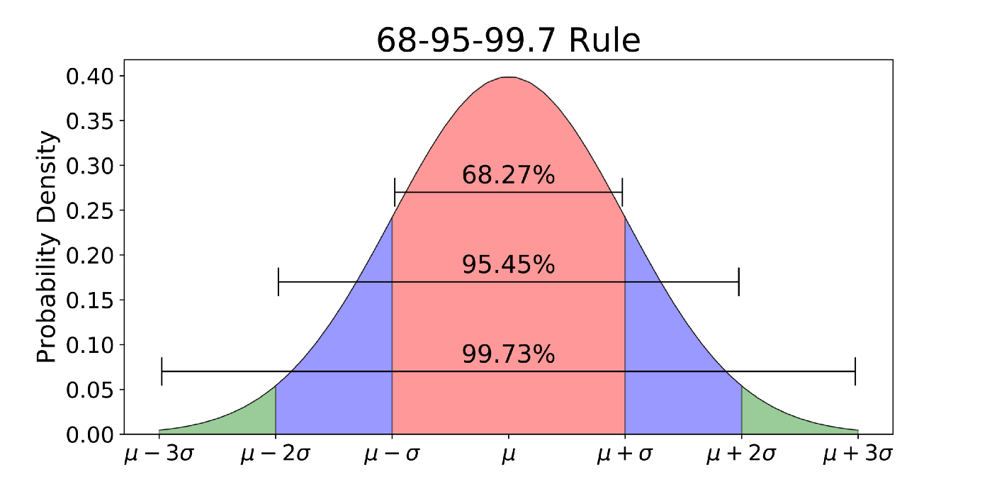
Figure 7.1 Histogram of normal distribution generated in snippet 7.1
There are two important parameters of normal distribution: mean and standard deviation. The mean of histogram from 7.1 is equal to 10 and the standard deviation is equal to 1.
Standard deviation is a very important measure of data spread. It is as important as the mean value, since it tells us how widely or narrowly data is spread around the mean. Mathematically, standard deviation is defined by the following formula:
\[\begin{equation} \sigma = \sqrt{\frac{\sum(x_i - \mu)^2}{N}}\\ \text{where:}\\ \sigma \text{= population standard deviation}\\ \text{N = the size of the population}\\ x_i \text{= each value from the population}\\ \mu \text{= the population mean}\\ \end{equation}\]
The squaring of differences between data points and the mean value is important since it treats negative and positive differences identically. Dividing by the number of data points is important for normalization.
Given a numerical variable x, sd(x) is the R function which computes standard deviation. It is demonstrated in the snippet 7.1
These will be useful later in hypothesis testing.
In the following snippet we use two functions rnorm() and pnorm(). Function rnorm() generates a number of data points according to normal distribution assuming the mean=10 and standard deviation (sd) =1. Normal distribution is the core distribution in data science (although power law distribution is also gaining ground as we explain in a separate section). Normal distribution plays a special role due to the Central Limit Theorem ??.
Feel free to change parameters of rnorm() in snippet 7.1 and see the effect of mean and standard deviation in the shapes of resulting bell curves.
The statement length(normal[normal >x]) shows the number of data points which are larger than x. In the snippet x=12. Notice how quickly length(normal[normal >x]) goes down to zero when one increases x. The statement z<-(12-10)/10 calculate the z-value, which is defined as difference between x and the mean of the distribution divided by standard deviation. This helps normalization and allows talking about vastly different data sets in the same terms.
Z-value is the distance measured in sigmas, where sigma stands for one standard deviation.
The function pnorm(z) calculates the fraction of data points in normal distribution whose z-value is less than z. Regardless of what standard deviation and mean of a given data set is, this fraction is always the same for the same values of z. Z-value is the common denominator normalizing all data distributions. With z-values we may disregard the range of data as well as its mean. It allows us to define distance from the mean in units which are standard deviations (sigmas).
The reader is encouraged to change all the parameters of this snippet and see the effect of z-value on the number of values exceeding z. This fraction becomes negligible roughly around z approaching 3. For z-values larger than 5, one cannot observe a single value with z>5, unless the data set is very large. Thus, the decline of the Gaussian Bell curve is very steep!
1-pnorm(z) returns the area under the bell curve with z value larger than z. In our case z=0.2. As you can check 1-pnorm(z) returns 0.42. Thus, 42% of the area under the bell curve is larger than z=0.2.